


Inside China’s Machine · Tokenomics, Episode 2 of 10
The Answer Price = price per token × tokens per attempt ÷ success rate
This episode: what it costs the provider to serve, underneath the price per token
When DeepSeek announced V3 in Chinese, the key line was short: “DeepSeek-V3 为自研 MoE 模型,671B 参数,激活 37B”. In English: an internally developed mixture-of-experts model with 671 billion parameters, 37 billion of them activated.
That sentence gives two sizes for one model. Read quickly, it sounds like a contradiction. Read slowly, it is the starting point for understanding what makes a model cheap or expensive to run.
The first episode of this series argued that the economic unit of machine intelligence is a successful task, not a token: what it costs to get a defined piece of work done and checked. This episode goes one layer down. Before a model is deployed on any hardware, at any price, its design already constrains how much computation and memory it needs to produce each token, at a stated context and precision. That is the floor everything above it is built on. And the floor turns out to have at least three separate parts.
The simplest case
Start with a plain model, the kind sometimes called dense. In simplified accounting, every counted weight is treated as taking part each time it produces a token. A hypothetical dense model with 70 billion parameters stores 70 billion parameters and uses 70 billion parameters per token. Its size is one number because the two quantities are the same.
In that simple world, a model’s size tells you two things at once: how much memory it takes to hold the model, and how much arithmetic each token needs. A bigger model costs more to store and costs more to run.
The designs in DeepSeek’s and Qwen’s own releases pull those two things apart and add a third that grows with use. Each design can change a different combination of them. To see what any of them does to cost, they have to be taken one at a time.
The weights a model uses
A mixture-of-experts model splits much of its network into many smaller sub-networks, the experts, and routes each token to only a few of them. The model stores all of the experts. For any one token, it calculates with only the selected ones.
Qwen3’s Chinese release puts numbers on this. Its larger model is described as having “2350 多亿总参数和 220 多亿激活参数”, over 235 billion total parameters and over 22 billion activated. Its smaller one has “约 300 亿总参数和 30 亿激活参数”, about 30 billion total and 3 billion activated. The architecture table in the same release gives both models 128 experts, of which 8 are activated.
Qwen3-Coder-Next, a coding model from the same team, goes further: its model card lists 80 billion parameters in total and 3 billion activated.
Divide the active count by the total and the fractions are small. For DeepSeek-V3 it is about 5.5 percent. For Qwen3’s larger model, about 9.4 percent. For Coder-Next, 3.75 percent.
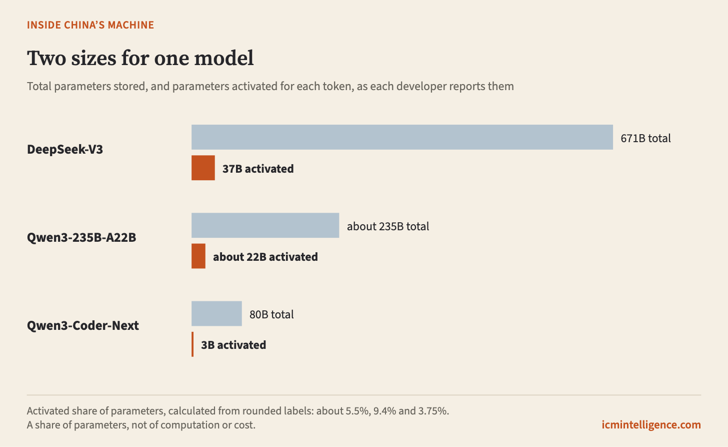
Those percentages are easy to misread, so it is worth saying what they are. They are fractions of parameters, calculated from rounded labels. They are not the share of all the computation a token needs, because routing, attention and other operations sit outside the expert weights. They are not speedups. They are not cost reductions. What they do show is that for the expert layers, the arithmetic per token is tied to the active count, not the total.
The weights a model stores
The total count did not go away. A model that activates 37 billion parameters per token still has to keep all 671 billion somewhere, ready for whichever experts the next token selects.
In the simplest accounting, the memory needed just to hold the weights is the number of stored parameters times the bits used to store each one. A small active count therefore says little about storage. Coder-Next’s 3 billion active parameters sit inside an 80 billion parameter model.
This is the first split that matters for cost. Arithmetic per token follows the active weights. Memory to hold the model follows the total weights. The two can move in different directions, and they bind different resources. How a deployment arranges the stored weights across machines is a question about serving, which the next episode takes up. At the model level, the point is narrower: “how big is it” now has two answers, and a cost estimate needs both.
The memory a model keeps for each token
There is a third quantity, and it grows with use. When a model reads a long prompt or writes a long answer, it keeps a record for every token so far, so that each new token can attend back to the earlier ones. That record is usually called the key-value cache. A longer conversation means a bigger cache.
DeepSeek’s design compresses it. Its technical report describes an attention method called MLA, built on “low-rank joint compression” of the keys and values. The saving is easiest to see as storage. In standard attention, every past token leaves behind a full key and a full value for each attention head. DeepSeek-V3 has 128 heads of 128 numbers each, so keeping all of them would take 32,768 numbers per token in every attention layer. MLA keeps something much smaller: one compressed vector of 512 numbers that summarizes the token’s keys and values, and a separate key of 64 numbers that records the token’s position. Added together, that is 576 numbers kept per token for each attention layer.
The full keys and values are not lost. When the model needs them, it rebuilds them from the compressed vector, using what the report calls “up-projection matrices”. Those matrices are part of the model’s weights: the same for every token, and stored once with the rest of the model. The cache therefore holds only what is unique to each token, its 576 numbers. The report lists those two vectors as the only things that “need to be cached during generation”. A token’s query is used only while that token is being produced, so it is never stored.
That figure is a count of numbers, not of bytes. How many bytes it becomes depends on the precision used to store them, the number of layers and the length of the context, none of which this figure fixes. It also excludes the temporary memory any real system needs. But it shows where the design aims its saving: a short summary for each past token, instead of a full key and value for every head.
DeepSeek has said the same thing in Chinese, in an announcement about its API’s disk cache: “这得益于 DeepSeek V2 提出的 MLA 结构”, this benefits from the MLA structure introduced in DeepSeek V2, which “大大压缩了上下文 KV Cache 的大小”, greatly compresses the size of the context KV cache.
So the third requirement is the memory per token of context. It is separate from the active weights and separate from the stored weights. A model can be small in arithmetic per token and still carry a large cache on a long task, or the reverse.
Fewer bits per number
One more lever changes none of these counts, only how precisely each number is written down.
DeepSeek’s Chinese release states that V3 “采用 FP8 训练,并开源了原生 FP8 权重”: it was trained in FP8, an 8-bit number format, and its weights were released in native FP8. The technical report adds that the training framework keeps some sensitive components in their “original precision”. Lower precision is a deliberate choice applied selectively, not a setting applied to everything. Qwen publishes an FP8 version of Qwen3-14B; its card describes “fine-grained fp8 quantization with block size of 128.”
In the simplest accounting, fewer bits per weight means less memory per weight. Going from 16 bits to 4 would cut the space needed for the weights themselves to a quarter, before counting the extra values that quantization schemes store alongside the weights, and before counting everything else in memory.
This is where quality comes in, and it is the first real test of the per-token saving. An independent study of quantized Qwen3 models reports the same 8-billion-parameter model on the MMLU benchmark. At 16-bit precision it scores 74.7. With its weights reduced to 8 bits by one method, GPTQ, it also scores 74.7. With its weights reduced to 4 bits by another method, AWQ, it scores 69.3: 5.4 points lower.
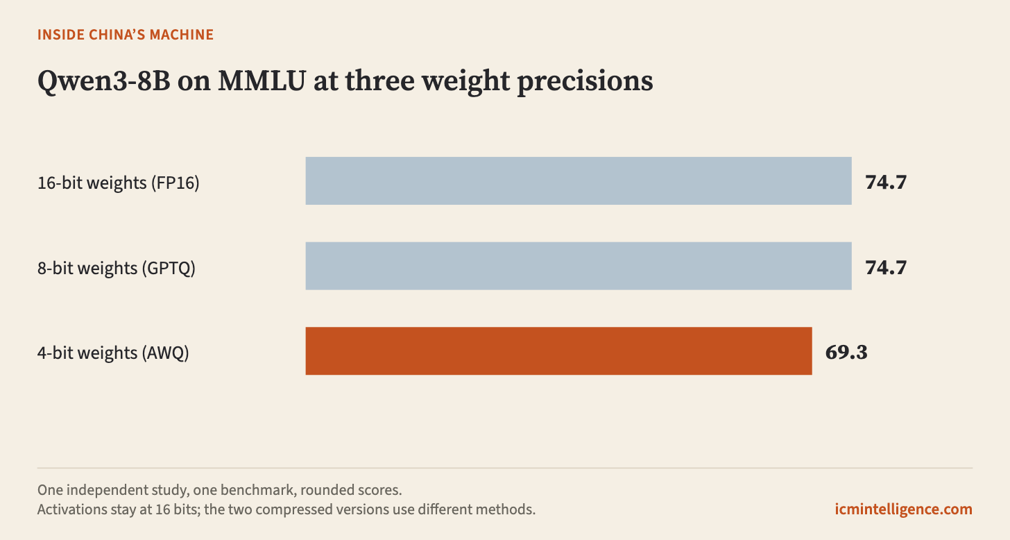
On that one benchmark, at the reported rounding, halving the bits left the score unchanged, and quartering them cost 5.4 points. The two compressed versions used different methods, so the comparison does not isolate bit width alone. It does show the general shape. A saving in memory per weight is real, and whether it survives depends on whether the answers stay good enough for the task.
Compute per task is a dial
Everything so far concerns what one token requires. A task requires many tokens, and how many is increasingly a choice.
Qwen3’s Chinese release describes two modes, “思考模式” and “非思考模式”, thinking and non-thinking, and says this flexibility “使用户能够根据具体任务控制模型进行“思考”的程度”, lets users control how much the model thinks according to the specific task. The technical report explains the mechanism: when the model’s reasoning reaches a “user-defined threshold”, the system will “manually halt the thinking process”, and the model then produces its final answer. Qwen reports that performance on its tested mathematics, coding and STEM benchmarks improves as the thinking budget grows.
That makes compute per task a dial rather than a property of the model. The same weights, with the same cache design, can spend more or fewer tokens on a question, depending on a setting. Not every model offers the dial: Qwen3-Coder-Next’s card says plainly, “This model supports only non-thinking mode”.
Research on this kind of spending adds two cautions. The final ICLR 2025 version of the paper by Charlie Snell and co-authors on scaling computation at answer time finds that its effectiveness “critically varies depending on the difficulty of the prompt.” And its own cost accounting is partial. To compare spending fairly, the authors count inference with a formula of “Y = 4ND inference”, where N is the model’s parameter count and D the number of tokens generated, instead of the “standard 2ND inference”, doubling it “to account for the overhead of calling the verifier”, an answer checker. They also note that one step, predicting how hard a question is, is left out: “Our experiments do not account for this cost largely for simplicity”. A full ledger of what a solved task consumes has to include the checking and the routing, not only the generation.
The floor, rebuilt
Put the pieces into the measure this series uses. The computation needed per successful task, over a fixed batch of tasks, is all the computation spent divided by the number of tasks that succeed. Broken into parts, it is the computation per token, meaning all counted computation divided by all counted tokens, times the average tokens per attempt, divided by the success rate.
Each design lever lands on a different term.
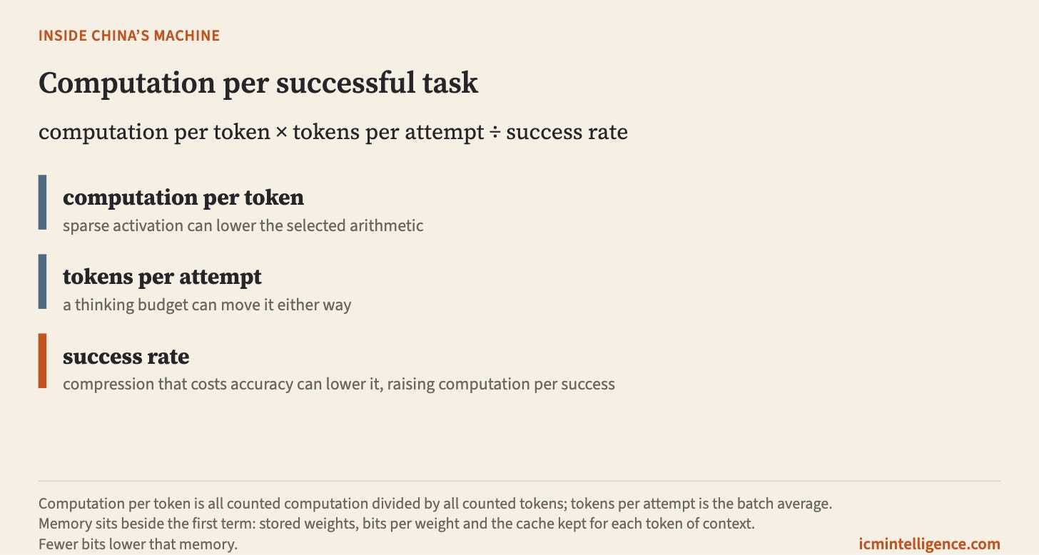
Sparse activation lowers the selected arithmetic in the first term, the work per token, while fewer bits and cache compression lower the memory that sits beside it. A thinking budget moves the second term, the number of tokens an attempt consumes, in either direction. Quality decides the third term: a cheaper model that fails more often needs more attempts per success.
So a per-token saving becomes a per-task saving only if changes in the other two terms do not fully offset it. If a lighter model needs more thinking to reach the same answer, the second term rises. If compression costs accuracy, the third term falls. The saving in the first term can survive, shrink or disappear, and only a measurement on a fixed task can say which.
Qwen3-Coder-Next shows why the question is worth asking. With 3 billion active parameters, it reports SWE-Bench Verified scores of 70.6 percent, 71.1 percent and 71.3 percent on three different agent frameworks, SWE-Agent, MiniSWE-Agent and OpenHands, with the number of agent turns capped at 300. That is substantial coding capability from a small active footprint. It is not a cost per solved problem. A cap of 300 turns says nothing about how many turns, or tokens, each problem actually used, and those are the numbers the second term needs.
The research behind this episode did not find an independent measurement that holds a useful task and its quality fixed and compares what these models consume to get it done. That is the gap between the mechanism and a cost claim.
The number that is not an inference cost
One DeepSeek figure belongs to a different ledger.
DeepSeek’s technical report gives the training of V3 as 2,664,000 H800 GPU-hours for pre-training, 119,000 for extending its context length and 5,000 for post-training: 2,788,000 in total. The report says these figures exclude the costs of “prior research and ablation experiments”.
That number describes the inputs to one training run. It is not the cost of running the model, which depends on how many requests it serves, how long they are and how often they succeed. Nor is it the full cost of building the model, by the report’s own boundary. Training cost and inference cost are separate systems. A low training figure can coexist with expensive inference, and the reverse. Neither prices a solved task.
China’s role, stated narrowly
The Chinese releases in this episode are evidence for the mechanism, read in the original: sparse activation, compressed attention memory, native 8-bit weights and a selectable thinking budget, each described by the teams that built them.
That is a real contribution to the economics of machine intelligence, and it should be stated no more broadly than the evidence allows. These documents describe designs. They do not show that export controls caused them. They do not show that Chinese models deliver a solved task more cheaply than others at matched quality; no such measurement appears in the evidence here. The models in this episode are named checkpoints, not a survey of the newest or cheapest.
What they do show is that the cost floor is no longer one number. A reader who hears “671 billion parameters”, “3 billion active” or “576 numbers cached per token in each layer” now knows to ask which of the three sizes is meant.