



Inside China’s Machine · Tokenomics, Episode 3 of 10
The Answer Price = price per token × tokens per attempt ÷ success rate
This episode: what it costs the provider to serve, underneath the price per token
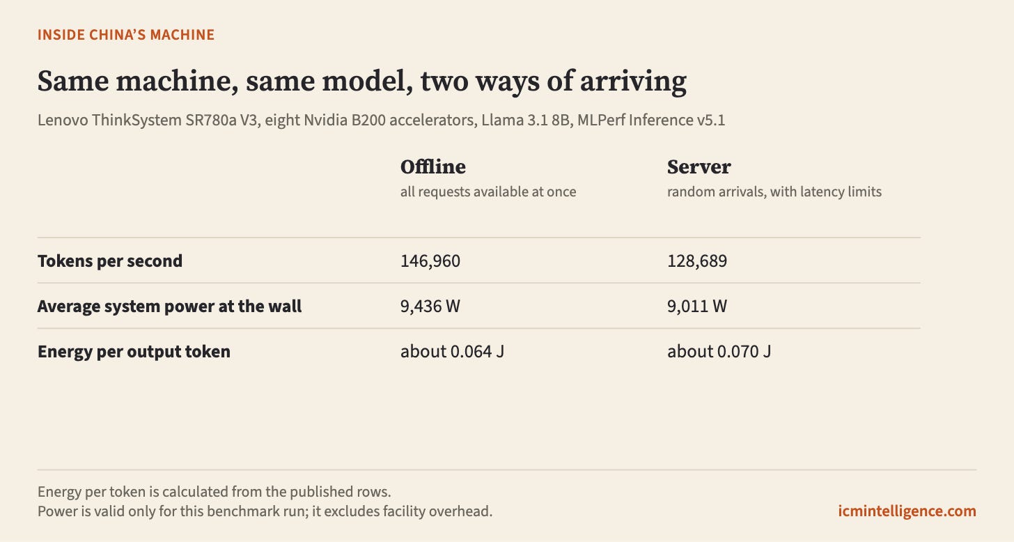
In the MLPerf inference benchmark, a Lenovo server with eight Nvidia B200 accelerators ran the Llama 3.1 8B model in two ways.
In the first, called Offline, all the requests are available at once and the system works through them as fast as it can. It produced 146,960 tokens a second while drawing an average of 9,436 watts at the wall.
In the second, called Server, requests arrive at random times, and the run is held to latency limits on how fast the answers come back. The same machine, the same model and the same software produced 128,689 tokens a second, drawing 9,011 watts.
Divide the power by the output and you get the energy behind each token: about 0.064 joules in the first case, about 0.070 in the second. The hardware did not change. The model did not change. What changed is how the work arrived and how fast it had to be answered.
Episode 2 looked at what a model needs per token: the weights it stores, the weights it uses, the memory it keeps for context. Now the model goes to work. Requirements are a floor, the least a model costs to run. Serving decides how far above that floor the bill lands, and the difference can be large enough to reverse a comparison.
The simplest case
Start with one server you pay for by the hour, whether you use it or not, and one job to run on it: pulling fields out of a document, about 2,000 tokens in and 500 out.
Over a month, the cost of that capacity is fixed. The cost per accepted task is that fixed cost divided by the number of tasks that pass. Double the work that passes and the cost per task halves. Leave the machine idle half the time and each task that does run carries the cost of the idle hours too.
That single division explains most of the economics of serving. A faster serving system lowers cost per task only if there is demand to fill the extra speed. A cheaper hourly rate lowers it only if the hours are used. And a task that fails still consumed capacity, so the denominator counts what passes, not what ran.
Four limits matter: how many requests one machine can carry at once, how fast it must answer, how much of its time is filled, and how much power it can draw.
Many requests on one machine
A serving system does not have to handle one request at a time. It groups them, so that one pass over the model’s weights serves many users at once. Grouping raises throughput, but in its simplest form it has a cost: a request may wait for its group to fill, and a group is only finished when its longest request is done.
Modern serving software works around both problems. vLLM, a serving engine, schedules work one step at a time. The paper that introduced vLLM describes the technique, continuous batching, in one line: “After each iteration, completed requests are removed from the batch, and new ones are added.” No group waits for its slowest member.
Memory is the other limit. Episode 2 described the cache a model keeps for every token of context, its running memory of the text it has already read. In a serving system, every request in flight needs its own share of that cache, and the cache has to fit in memory beside the weights. The vLLM team found that older systems wasted memory by holding back space for the longest answer a request might produce and by leaving gaps too small for any other request to use. Their answer, called PagedAttention, stores each request’s cache in small fixed-size blocks, so less is wasted and more requests fit.
The paper describing it reports throughput gains of 2 to 4 times “with the same level of latency” against earlier serving systems such as FasterTransformer and Orca, on its workloads. That result cuts against an easy assumption: that serving more requests at once must mean slower answers. Better software served more requests at the same reported latency level.
Sharing has a limit, though. The vLLM walkthrough describes the token-by-token generation phase as “memory-bandwidth-bound”: each new token requires reading the weights and the cached context again, and the time to move those bytes, not the arithmetic, sets the pace. Too many requests competing to read memory at once slows each of them.
How fast is fast enough
The second thing serving adds is a deadline: a limit on how long each answer may take to come back.
For language models, the benchmark’s rules measure two things: the time to first token, how long a user waits before anything appears, and the time per output token, how fast the answer flows after that. In the Server run, 99 requests in 100 got a first token within 1.026 seconds. Taken separately, at the 99th percentile the tokens that followed came on average every 27.1 milliseconds. The limits set for that test were 2 seconds and 100 milliseconds. The run passed.
The deadline matters because it decides how hard the machine can be pushed. A system extracting fields from documents overnight can run fuller and with larger groups. A system serving people who are waiting gets only as full as its latency limits allow. The two MLPerf scenarios show the same hardware delivering different throughput under the two regimes, though they do not show which part of the difference comes from batching alone.
For an economic comparison, this means a throughput figure means nothing without its deadline. MLCommons makes the same point about power: it measures the whole system at the wall, and a power result is valid only for the benchmark it accompanies. Move it to another model, another load or another machine and it no longer applies.
How much of the time is busy
The third thing is occupancy: how much of the paid capacity is busy.
This is where a direct measure is needed, and where it is easy to mistake one measure for another. To see what such a disclosure looks like in China, take the China Academy of Information and Communications Technology, CAICT, which gives a useful example of both what exists and what does not.
In a 2025 report on the compute economy, CAICT describes a cross-architecture scheduling case in which resource utilization reached 78 percent. That is a real disclosure, but it does not say how utilization was measured, over what period, or how much of it was accepted work. CAICT’s 2025 blue book on advanced computing, dated March 2026, cites industry-ministry data putting average rack occupancy near 60 percent.
Rack occupancy measures how many racks in a data centre are filled with equipment. It says nothing about whether the accelerators in those racks are busy, let alone busy with requests that passed. A data centre can be full of machines that sit idle. For the cost of a solved task, the measure that matters is demand occupancy: of all the work the installed machines could finish on time, how much is actually asked of them, with the success rate applied separately. Neither CAICT figure is that number.
Power, and compute sold as a service
Power enters twice. The first time, it is a bill: energy used, times the price of electricity, times the overhead of cooling and power delivery. That overhead is what power usage effectiveness, or PUE, measures: a PUE of 1.3 means 1.3 units of energy drawn for every unit that reaches the computers. The second time, it is a ceiling. A site can only run as many machines as it has firm electrical capacity for, and cheap electricity does not help if the power cannot be delivered when the machines need it.
China’s policy documents address both. A 2023 opinion from the National Development and Reform Commission steers eastern demand that can tolerate delay toward clean-energy-rich regions outside the national hubs; the next line names AI model training and inference among the eastern workloads to move west. A 2024 action plan sets PUE targets for new and expanded data centres. On price, Guizhou’s energy bureau reports, in its 2024 accounts, an electricity price of 0.3515 yuan per kilowatt-hour for large data centres in Gui’an, and credits the low price to power-supply subsidies to generating companies.
These are targets, requirements and one local outcome. None of them measures what the fleet achieved or shows that useful work is cheaper there once latency, delivered capacity and everything else are counted, and the Guizhou figure is historical, local and tied to a policy: it is not a national tariff.
CAICT also describes a shift in China’s compute from selling hardware toward service subscriptions, delivered in the form of a service such as an API, with computing, storage and networking bundled together. When the buyer pays per use, the occupancy risk sits with the provider, which needs enough demand to keep its machines busy. None of this shows Chinese compute is cheaper per solved task. Whether these levers deliver cheaper accepted work at matched quality and deadlines remains open until it is measured.
When renting the machine beats buying the answer
All of this comes together in a practical choice: pay an API provider per token, or run the model yourself on rented or owned hardware.
Take a small cost model of that choice, built from public prices and stated assumptions. Its inputs are real list prices: Together AI charges $0.14 per million input tokens and $0.14 per million output tokens for Llama 3 8B Instruct Lite, and Runpod displayed an H100 SXM with 80 gigabytes of memory at $3.49 an hour, on a page updated September 27, 2026. Everything else is assumed and stated: a document-extraction task of 2,000 input and 500 output tokens, a 90 percent success rate on both routes, a deadline the self-run machine is assumed to meet at eight completed attempts a second, a 25 percent markup on the rental bill for spare capacity, such as a standby machine for failover, and monthly allowances for engineering, security, integration and storage. The results are modeled, not measured.
On the API, one attempt costs $0.00035 in tokens. The cost model then adds an assumed $0.002 per attempt for reviewing the output on both routes, which is larger than the token bill itself. That makes $0.00235 per attempt. Since only 90 percent of attempts pass, every accepted task also carries the cost of the attempts that failed: divide by 0.9, and the API comes to about $0.00261 per accepted task. The same division applies to the rented machine. Renting a machine costs a fixed $4,741 a month in this cost model, whatever the volume: $3,141 for 720 rented hours at $3.49 plus the 25 percent spare-capacity markup, and $1,600 of assumed allowances for engineering, security, integration and storage.
That fixed bill is spread over the documents the machine handles, so the cost of each accepted task falls as the machine fills. At 10 percent occupancy the rented machine costs about $0.0048 per accepted task, against about $0.00261 on the API. At 50 percent it costs about $0.0027, and at 75 percent about $0.00256, just under the API.
The two routes cost the same at about 13.5 million attempts a month. On the assumed throughput, that is about 65 percent occupancy of the rented machine. Below that, the API is cheaper per accepted task. Above it, renting wins. The rental bill already includes the 25 percent markup, which pays for standby capacity in case the machine fails. That is separate from demand: the cost model also treats the machine as full at 80 percent occupancy, keeping the rest free for bursts. The markup raises the cost; the cap limits the volume.
Owning means buying the machine and paying for its power; the cost model spreads the purchase price over the machine’s life, which gives a fixed monthly cost of $3,149 against $4,741 for renting. Owning therefore breaks even earlier, at about 9.4 million attempts, or 45 percent occupancy.
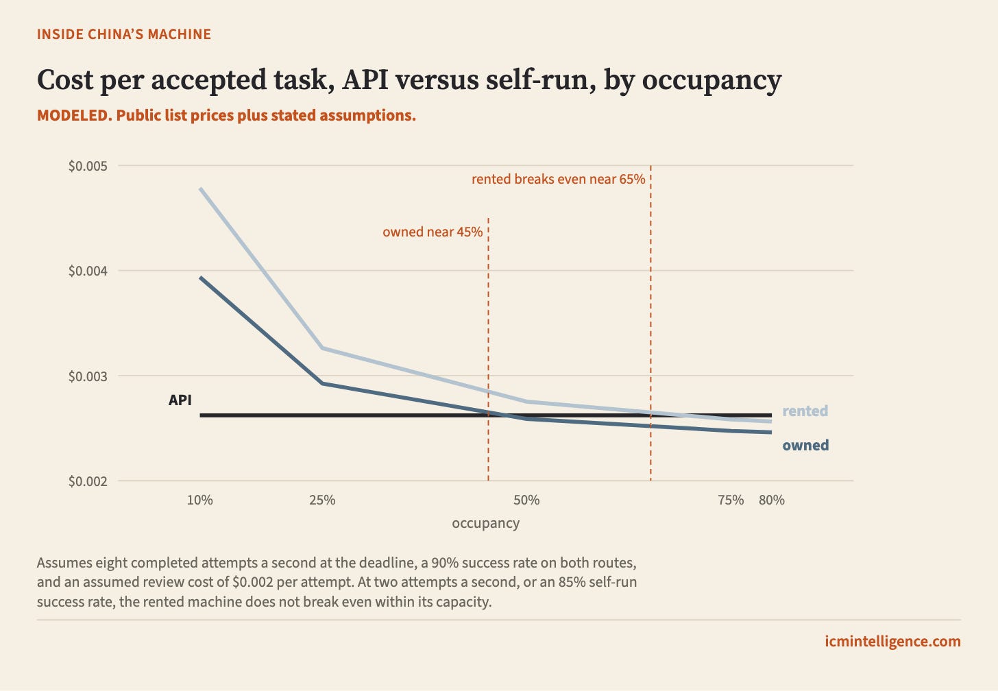
Then the assumptions move, and the crossover moves with them. If the machine can only complete two attempts a second at the deadline instead of eight, renting never catches the API on one machine: the break-even volume would need more than twice the machine’s capacity. If the self-run success rate is 85 percent instead of 90, while the API keeps its 90 percent, the rented machine cannot reach break-even within its capacity either. If the API price halves, the same happens.
The variable-cost saving from renting is thin in this cost model, about $0.00035 per attempt, the token bill it avoids, before the fixed monthly bill is counted, which is why small changes in speed, success or price can erase it. None of these numbers is a forecast or a ranking. The cost model is arithmetic on assumed inputs, and whether the same AI model at the same precision would pass at the same rate on both routes is untested. What the cost model shows is the shape of the answer. The crossover depends on throughput at a deadline, on occupancy and on success rate, and it is narrow: renting wins only between about 65 and 80 percent occupancy, by less than 3 percent per task, and a modest change in any of them can erase it.